Investigation of the Erdos–Renyi model

A post by Roman Zhuravel and Guy Koplovitz

We investigated the Erdos–Renyi model by simulating random non-directional graphs and counting (and visualizing) the number of graphs connected-components.
​

Erdos–Renyi model

This model describes the behavior of components' number and size in a graph G(n, p), when n→inf. The graph is constructed by connecting nodes randomly, i.e. Each edge is included in the graph with probability p, independent of every other edge. The behavior of random graphs is often studied in the case where n, the number of vertices, tends to infinity. Although p can be fixed in this case, it may also be defined as a function which depends on n. For example, the statement:

• Almost every graph in G(n, 2ln(n)/n) is connected.

Which means that as n tends to infinity, the probability that a graph, of n vertices with edge probability of 2ln(n)/n, is connected tends to 1.

Properties of G(n,p)

In a 1959 paper[1], Erdos and Renyi described the behavior of G(n,p) very precisely for various values of p. Their results included:

• If np < 1, then a graph in G(n,p) will almost surely have no connected components of size larger than O(log(n)).
• If np = 1, then a graph in G(n, p) will almost surely have a largest component whose size is of order n^(2/3).
• If np →c>1, where c is a constant, then a graph in G(n,p) will almost surely have a unique giant component containing a fraction of the vertices. No other component will contain more than O(log(n)) vertices.
• If p< (1- ε)ln(n)/n, then a graph in G(n, p) will almost surely contain isolated vertices, and thus be disconnected.
• If p>(1+ ε)ln(n)/n, then a graph in G(n, p) will almost surely be fully connected.

Thus p=ln(n)/n is a sharp threshold for the connectedness of G(n,p).

In this exercise we simulate random graphs to check the last conclusion from the paper of Erdos and Renyi: the p = ln(n)/n threshold theorem.
The simulation is done as follow:

• Create random graphs with n vertices and edge probabilities of p
• Calculate the number of components in the graph
• Average the results over many graphs (100) with the same n & p
• Compute the average number of components for various n's and p's
• Plot a 3D graph of the average number of components as a function of n & p
• Plot on top of the 3D graph the  threshold line

In addition we present representative random graphs for chosen n & p and differentiate between components by coloring the connected components with the same color.

Results

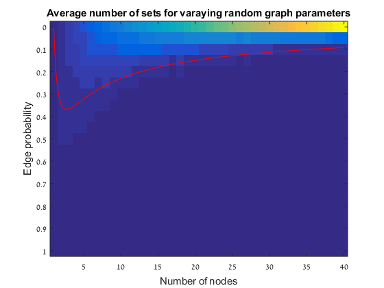
The red line is the p  = ln(n)/n threshold which shows that the simulation follows the theory quite nicely.

Representative random graphs
Since those graphs are random, they might diverge from the averaging map above.
For n = 10 & p = 0.15 :

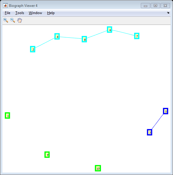
For n = 20 & p = 0.1:

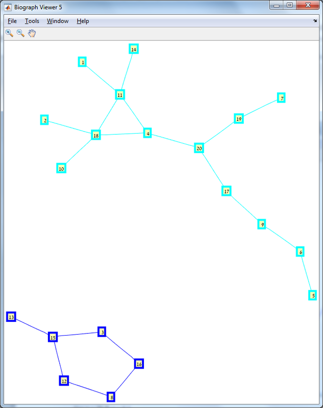
For n = 40 & p = 0.02:

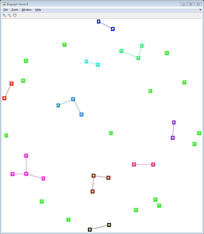
Methods

For this exercise we used the biograph object which is a part of Matlab's Bioinformatics Toolbox.
In order to expedite long calculations we applied Matla's parallel computing capabilities.

[1] - ERDdS, P., and A. R&WI. "On random graphs I." Publ. Math. Debrecen 6 (1959): 290-297.‏